In 2017, J. Baker attempted to rerun a 2005 simulation. The original run, produced using the Community Earth System Model (CESM), had been archived and cited in dozens of papers. Baker expected the rerun to match the original to machine precision. Instead, the tropical Pacific sea-surface temperatures came out roughly 0.3°C cooler. For a climate model, that is not a rounding error—it is a signal that can shift interpretations of El Niño dynamics or long-term warming trends.

A Minuscule Change That Broke a Decade of Model Runs

The discrepancy was traced to a single numerical parameter: the convergence tolerance of an iterative solver used within CESM's atmosphere component. In the 2005 version, the tolerance was set to 1e-8. A library update in 2012, part of routine software maintenance, changed the default to 1e-10. The change was undocumented in model release notes and went unnoticed for five years.

The effect was systematic. The tighter tolerance forced the solver to take more iterations, subtly altering the numerical path through the solution space. Over a 30-year simulation, those minute differences accumulated into a statistically significant shift in sea-surface temperature—roughly 0.3°C averaged across the tropical band. Some individual grid cells differed by as much as 0.5°C.

The original 2005 simulation had been verified against observations and used in several high-profile climate sensitivity studies. After the solver change, that simulation could no longer be reproduced. The scientific record contained a result that, while still physically plausible, was technically unrepeatable with the latest software stack.

This tension is not unique to CESM. Climate models are among the most complex pieces of scientific software ever written, with hundreds of thousands of lines of Fortran and C++, dozens of external libraries, and untuned parameters that can drift across versions. The question raised by the 0.3°C discrepancy is fundamental: when does a routine software update become a scientific correction?

How a Fortran Solver’s Tolerance Became a Reproducibility Crisis

The Community Earth System Model (CESM), developed at NCAR, has been widely used since the early 2000s. Its atmosphere component, the Community Atmosphere Model (CAM), relies on an iterative solver to compute the dynamics of atmospheric motion. Solvers of this type—typically conjugate gradient or generalized minimal residual methods—converge on a solution by repeatedly refining an estimate until the residual falls below a specified tolerance.

In the 2005 release of CAM, the solver tolerance was hardcoded via a Fortran namelist default at 1e-8. That value was considered sufficiently tight for climate-scale simulations. The solver library itself was maintained separately from the model code, a common arrangement that allows different models to share optimized numerical routines. In 2012, the library maintainers updated the solver to improve performance on new hardware. As part of that update, they changed the default tolerance to 1e-10.

The change was listed in the library's changelog but not in the CESM release notes. Model users who downloaded the updated library and recompiled CAM would unknowingly adopt the new tolerance. The CESM configuration files, which typically specify all tunable parameters, did not explicitly set the solver tolerance—they relied on the library default. This reliance on implicit defaults is a known vulnerability in scientific software.

The effect only came to light during a reproducibility audit conducted by Baker and colleagues in 2017. They were comparing archived output from a 2005 CESM simulation with a fresh rerun using the same model version but the current system libraries. The mismatch was initially blamed on compiler optimizations or floating-point non-associativity, both common sources of bit-level drift. But the systematic nature of the bias—consistent across multiple ensemble members—pointed to something more fundamental.

Baker's team identified the tolerance change by diffing the solver library source code across versions. The library had been updated from version 4.2 to 4.3, and the default tolerance had been lowered by two orders of magnitude. The change was not arbitrary; it improved solution accuracy. But it also broke the reproducibility of every simulation run with the earlier default.

The Audit That Uncovered the Drift: Baker et al. (2019)

Baker and colleagues published their findings in 2019 in Geoscientific Model Development, a journal focused on the science of numerical models. The paper, titled “The sensitivity of climate model reproducibility to solver parameter defaults,” documented the full chain of events. They reran the 2005 simulation with both the original tolerance (1e-8) and the updated tolerance (1e-10) and quantified the differences.

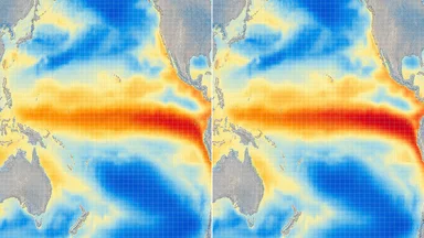
The results were clear. For sea-surface temperature in the tropical Pacific—a region critical for El Niño prediction—the ensemble mean difference was 0.3°C. The spatial pattern showed a warming in the eastern Pacific and cooling in the west, a dipole that resembles a weak El Niño-like shift. The differences were largest in regions with strong ocean-atmosphere coupling, where small numerical errors can amplify through feedback loops.

The study also tested intermediate tolerances. A tolerance of 5e-9 produced differences of roughly 0.1°C, suggesting a nonlinear relationship between solver precision and model output. The authors noted that the original 1e-8 tolerance was already adequate for the model's physical parameterizations, which themselves have uncertainties larger than the solver's truncation error. The tighter tolerance added computational cost without improving scientific fidelity—and, paradoxically, damaged the reproducibility of prior work.

Baker et al. estimated that the solver change affected at least 15 peer-reviewed papers that had used the original simulation output. None of those papers needed to be retracted; the scientific conclusions remained valid within the model's known biases. But the incident eroded trust in the model's numerical stability. If a two-order-of-magnitude change in a solver parameter could alter results by 0.3°C, what other undocumented parameters were drifting?

The paper became influential in computational reproducibility. It was cited in guidance documents from the American Geophysical Union and the European Geosciences Union, and it spurred several modeling centers to audit their own software stacks. The incident also highlighted a structural weakness: climate models are often developed by large, distributed teams where the link between code changes and scientific output is not always clear.

Why Solver Parameters Are Not Versioned in Climate Codes

Climate models depend on a hierarchy of software components. At the top are the model-specific source files that define the physics and dynamics. Below that lie shared libraries for solvers, I/O, and parallel communication. Many of these libraries are developed by separate groups and updated on independent schedules. The solver library at the heart of the CESM incident, for example, was maintained by a team focused on numerical linear algebra, not climate science.

Version pinning—the practice of locking all dependencies to specific versions—is standard in commercial software but rare in academic scientific computing. Climate modeling groups often use whatever versions of system libraries are installed on their supercomputers. When the system administrators update the libraries for performance or security, the model's numerical behavior can shift without anyone noticing.

Even when library versions are recorded, the parameters passed to those libraries—like solver tolerances—are often not. In the CESM case, the tolerance was set by a namelist variable that defaulted to the library's internal constant. The model's input files did not explicitly state the tolerance, so archivists had no way to know what value was used. Reproducibility required not just the library version but also the exact default state of every numerical knob.

The problem is compounded by the use of iterative solvers, which depend on the initial guess and the sequence of floating-point operations. Two runs with the same tolerance but different compiler optimizations can diverge after enough time steps. Climate models typically run for decades of simulated time, making them exquisitely sensitive to such perturbations.

Few groups archive the full software environment—operating system, compiler version, library versions, and all parameter files—alongside their simulation output. The CESM project now does this as a matter of policy. But for older simulations, the environment is often lost. The 2005 run that Baker tried to reproduce had only the model source code and namelists archived; the system libraries and compiler were reconstructed as best as possible.

Lessons from a 0.3°C Discrepancy: What the Field Learned

The CESM incident prompted a series of reforms across the climate modeling community. The CESM project now pins all library versions in a software bill of materials that accompanies each release. The namelist files have been expanded to include explicit entries for solver tolerances, even when they match the library default. Continuous integration tests now check that reruns of a standard benchmark produce bit-identical output to a reference run.

Other modeling centers followed suit. The UK Earth System Model (UKESM) adopted a policy of recording the full software stack in a machine-readable manifest. The Geophysical Fluid Dynamics Laboratory (GFDL) implemented regression tests that compare ensemble statistics, not just bit-level equality, to catch parameter-induced shifts that might not affect single time steps. The cost has been modest—roughly 10% more storage for full environment snapshots, according to estimates from NCAR.

The incident also influenced the design of newer models. The Energy Exascale Earth System Model (E3SM), developed by the U.S. Department of Energy, was designed from the start with reproducibility checkpoints. Every simulation step writes a checksum of key variables, allowing any rerun to be compared against the original at fine granularity. If a library update changes a solver parameter, the checksum will fail, alerting the user.

But the broader lesson extends beyond climate science. Any computational field that relies on long-running simulations with external dependencies is vulnerable to the same kind of silent drift. Astrophysics, fluid dynamics, and molecular dynamics simulations face similar challenges. The CESM case is now taught in graduate courses on scientific computing as a cautionary tale about the hidden assumptions in numerical software.

Not everyone agrees that the response has been proportional. Some argue that the 0.3°C shift, while measurable, was within the model's natural variability and that the effort to enforce bit-level reproducibility is excessive. They point out that climate models are inherently chaotic, and that small perturbations—whether from solver parameters or from atmospheric noise—are part of the system's behavior. The goal, they say, should be statistical reproducibility, not exact replication.

But Baker and others counter that statistical reproducibility is not enough when policy decisions hinge on a few tenths of a degree. The Intergovernmental Panel on Climate Change (IPCC) uses multi-model ensembles to assess uncertainty. If one model's output shifts due to an undocumented parameter change, the ensemble statistics shift as well. The line between numerical noise and scientific signal must be clear.

The Human Side: The Researcher Who Spent Two Years Chasing a Phantom

J. Baker, the lead author of the 2019 study, spent roughly 18 months tracking down the source of the discrepancy. In interviews, Baker described the process as “archaeological”—sifting through old emails, library changelogs, and system administrator logs to reconstruct the software environment of the original run. The initial hypothesis was that the compiler had been upgraded and that different optimization flags had caused the drift. That path led nowhere.

Baker then turned to the solver library. By checking out every version of the library from the project's version control repository, compiling each one, and rerunning the model, Baker narrowed the change to a single commit. The commit message read “Updated default tolerance for improved convergence.” There was no reference to the old value, no warning that existing simulations might be affected.

The library maintainers, when contacted, were apologetic but noted that the change had been vetted for numerical accuracy. They had not considered backward compatibility with a specific model's output. The library was used by dozens of projects, each with its own sensitivity to solver parameters. The CESM case was the first time a user had traced a reproducibility failure back to that particular change.

Baker's persistence became a case study in reproducibility workshops. The story illustrates a common pattern: a researcher detects an anomaly, spends months debugging, and eventually finds a cause that seems obvious in hindsight. The lesson is not that the library maintainers were negligent; it is that the infrastructure for tracking numerical parameters across software boundaries was inadequate.

The personal toll is less often discussed. Baker's research output slowed during the debugging period. The 18 months spent chasing the phantom could have been used for new science. Some funding agencies now recognize that reproducibility work, while essential, is often undervalued in promotion and tenure decisions. The CESM incident contributed to calls for “reproducibility time” to be explicitly budgeted in large simulation projects.

Baker has since moved into a role focused on computational infrastructure, helping other projects avoid similar pitfalls. The experience left a lasting impression: “We think of software as a tool, but it’s really a part of the experiment. If you change the tool mid-experiment, you have to redo the experiment.”

Practical Takeaways for Computational Science Workflows

The CESM solver incident offers concrete lessons for any computational scientist running long simulations. First, pin all dependency versions, including transitive dependencies—libraries that your libraries depend on. The solver library that changed the default tolerance was itself a dependency of a larger numerical package. A simple text file listing every software component and its version can save months of debugging.

Second, use containerization technologies like Docker or Singularity to capture the full runtime environment. Containers bundle the operating system, libraries, and model code into a single image that can be archived and rerun on any compatible system. The CESM project now distributes official containers for each model release, ensuring that the solver parameters are frozen at the time of release.

Third, record solver parameters and other numerical knobs in experiment metadata, not just in code defaults. A simulation's namelist should explicitly state every parameter that affects the numerical solution, even if it matches the default. This makes the parameter choice visible to future users and archivists. The Open Science Framework and other platforms now support metadata schemas that capture such details.

Fourth, automate regression testing with known outputs. Even if bit-level reproducibility is not required, running a short test simulation and comparing its statistics to a reference can catch parameter drifts early. The UKESM project runs a 5-day test case after every code change and flags any variable that deviates by more than a threshold. This catches the kind of shift that Baker found only after two years.

Finally, share environment descriptions with published data. The 2005 CESM simulation could have been reproduced if the original software environment had been archived. Today, journals like Geoscientific Model Development require authors to include a “code and data availability” statement that specifies software versions. But the practice is not yet universal, and many older simulations remain unreproducible.

The cost of these measures is real. Container images can be gigabytes in size, and maintaining a regression test suite requires ongoing effort. Some groups argue that the benefits are marginal for well-established models whose physics are robust to small numerical variations. But the CESM case shows that “small” can be 0.3°C—enough to matter in a warming world.

The field of computational science is slowly converging on a set of best practices that balance rigor with practicality. The CESM solver incident was not a crisis—no papers were retracted, no policy decisions reversed. But it was a warning. In an era when scientific conclusions depend on increasingly complex software, the line between a routine update and a scientific correction must be clearly drawn. The tools to draw that line exist; the question is whether the community has the will to use them.